3D Scene Graph Filtering using Graph Neural Networks

The core problem: too much context kills grounding

“Make me a meal” is a simple instruction for a human. For a robot it is an open-ended affordance query — no explicit object, no explicit room, no action sequence. Modern Vision–Language Models (VLMs) have dramatically improved the ability to interpret these queries, but they hit a hard wall when fed an entire 3D scene graph.

A typical indoor scene (from the Habitat-Matterport 3D Semantics dataset used here) contains ~661 distinct objects across ~106 categories. Serialising the full graph into a VLM prompt causes two distinct failure modes:

Context pressure. Relevant objects compete with noise for limited attention.
Hallucination. Confronted with hundreds of marginally-related facts, the VLM starts confidently inventing relationships that were never in the graph.

The second failure is the more dangerous one. More context is not free — it actively degrades grounding.

The solution: filter first, then reason

The thesis proposes inserting a learned Graph Neural Network filter between perception and the planner. The GNN reads the full scene graph together with the task query and assigns each node a relevance score. Only the high-scoring subgraph is forwarded to the VLM.

3D Mesh  ──►  Feature Extraction  ──►  Graph Neural Network  ──►  Filtered Graph
Task     ──►  Encoding Nodes      ──►  (Heterogeneous GAT)   ──►  VLM Planner  ──►  Plan
              └── 3D Scene Graph ──┘

This decomposition lets the VLM receive a small, grounded subgraph and spend its entire capacity on actual planning.

Background: the theoretical building blocks

Scene Graphs

A 3D scene graph $G = (V, E)$ is a hierarchical structure with three semantic layers:

Leaf nodes — individual objects (chair, mug, table…) with image and location attributes
Intermediate nodes — rooms and floors (living room, bedroom…) with category labels
Root node — the building itself
Edges — spatial/semantic relationships (object in room, room on floor)

Generation pipelines (Hydra, Kimera) process LIDAR/RGB-D data through 3D point-cloud segmentation, then build the graph by connecting nodes according to spatial coordinates and visual similarity.

Graph Attention Networks (GAT)

GATs are the core message-passing primitive used throughout this work. Given a graph $G = (V, E)$ with node features $X \in \mathbb{R}^{N \times F}$ :

Linear feature transformation:

h'_i = \mathbf{W} h_i, \quad \mathbf{W} \in \mathbb{R}^{F \times F'}

Attention coefficient between node $i$ and neighbour $j$ :

e_{ij} = \text{LeakyReLU}\!\left(\mathbf{a}^\top [h'_i \| h'_j]\right)

where $\mathbf{a} \in \mathbb{R}^{2F'}$ is a learnable attention vector and $\|$ denotes concatenation.

Softmax normalisation over the neighbourhood $\mathcal{N}(i)$ :

\alpha_{ij} = \frac{\exp(e_{ij})}{\sum_{k \in \mathcal{N}(i)} \exp(e_{ik})}

Feature aggregation via message passing:

h''_i = \sigma\!\left(\sum_{j \in \mathcal{N}(i)} \alpha_{ij} h'_j\right)

For $K$ attention heads, features are either concatenated or averaged:

\mathbf{h}''_i = \Bigg\|_{k=1}^{K} \sigma\!\left(\sum_{j \in \mathcal{N}(i)} \alpha^k_{ij} \mathbf{h}^{k'}_j\right) \quad \text{or} \quad \mathbf{h}''_i = \frac{1}{K}\sum_{k=1}^{K} \sigma\!\left(\sum_{j \in \mathcal{N}(i)} \alpha^k_{ij} \mathbf{h}^{k'}_j\right)

Heterogeneous GNNs

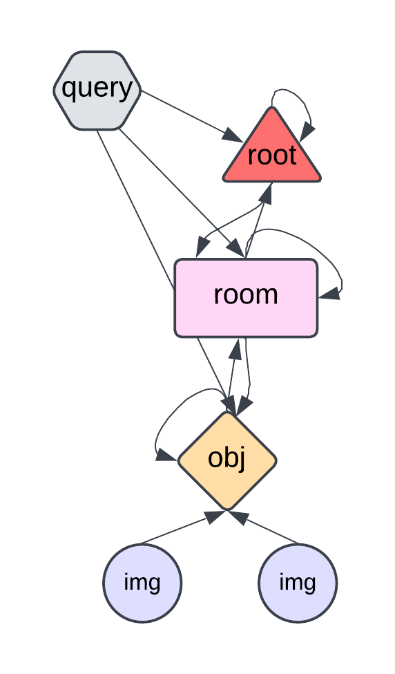
Because the scene graph contains different node types (object, room, root, image, query) and different edge types, a standard homogeneous GNN cannot be applied directly. The heterogeneous extension defines:

G = (V, E, \mathcal{T}_V, \mathcal{T}_E)

where $\mathcal{T}_V$ is the set of node types and $\mathcal{T}_E$ is the set of edge types.

Node representation update at layer $t+1$ :

h_v^{(t+1)} = \sigma\!\left(W_{t_v} h_v^{(t)} + \sum_{t_e \in \mathcal{T}_E} \text{Aggregate}_{t_e}\!\left(\{h_u^{(t)} : u \in \mathcal{N}_{t_e}(v)\}\right)\right)

Edge-specific aggregation for edge type $t_e$ :

m_{t_e}(v) = \text{Aggregate}_{t_e}\!\left(\{W_{t_e} h_u^{(t)} : u \in \mathcal{N}_{t_e}(v)\}\right)

Final node embedding combining all edge-type messages:

h_v^{(t+1)} = \sigma\!\left(\sum_{t_e \in \mathcal{T}_E} m_{t_e}(v) + W_{t_v} h_v^{(t)}\right)

Foundation models used for node encoding

CLIP

CLIP aligns image and text in a shared latent space via contrastive learning. Given image $I$ and text $T$ :

z_i = f_I(I), \quad z_t = f_T(T)

Cosine similarity:

\text{sim}(z_i, z_t) = \frac{f_I(I) \cdot f_T(T)}{\|f_I(I)\| \, \|f_T(T)\|}

Symmetric contrastive loss (logits $l_{ij} = \tau \cdot \text{sim}(z_i, z_t)$ ):

\mathcal{L}_{ITC} = -\frac{1}{N}\sum_{i=1}^N \log \frac{\exp(l_{ii})}{\sum_{j=1}^N \exp(l_{ij})}, \quad \mathcal{L}_{TIC} = -\frac{1}{N}\sum_{i=1}^N \log \frac{\exp(l_{ii})}{\sum_{j=1}^N \exp(l_{ji})}

\mathcal{L} = \frac{1}{2}(\mathcal{L}_{ITC} + \mathcal{L}_{TIC})

Used in this work: CLIP ViT-L/14@336px (768-dimensional embeddings).

BLIP-2

BLIP-2 introduces a lightweight Querying Transformer (Q-Former) that bridges a frozen image encoder and a frozen LLM. Three training objectives:

ITC Loss — aligns query embeddings with text in shared latent space:

\mathcal{L}_{ITC} = \frac{1}{N}\sum_{i=1}^N \left[-\log\frac{\exp(\text{sim}(z_i, z_t^+))}{\sum_{j=1}^N \exp(\text{sim}(z_i, z_t^j))} - \log\frac{\exp(\text{sim}(z_t, z_i^+))}{\sum_{j=1}^N \exp(\text{sim}(z_t, z_i^j))}\right]

ITM Loss — fine-grained image–text alignment:

\mathcal{L}_{ITM} = -\frac{1}{N}\sum_{i=1}^N \left[y_i \log p(y_i | z_i, z_t) + (1 - y_i)\log(1 - p(y_i | z_i, z_t))\right]

Used in this work: BLIP-2 with ViT-L/14 — the first query feature from 32 learned Q-Former queries produces image embeddings $h_i \in \mathbb{R}^{1 \times 768}$ . Text embeddings are the [CLS] token from the text encoder: $h \in \mathbb{R}^{1 \times 768}$ .

Approach

Problem definition

Formally: given a hierarchical 3D scene graph $G$ with nodes $N$ (carrying object images as attributes) and a task query $Q$ , find a subgraph $H$ with nodes $M \subseteq N$ such that the set of planning-critical nodes $O \subseteq M$ .

The filter must retain all objects needed to construct a plan while discarding as many irrelevant ones as possible.

Data generation pipeline

Step 1 — Visual data collection (Algorithm 1): For each object in Habitat-Sim, a robot navigates to randomised viewpoints:

R_{pos} \leftarrow \text{get\_nearest\_traversible\_pos}(pos, r', \theta', \phi')

where $r' \sim U(0.5,4) \cdot r$ , $\theta' \sim U(-90,90) + \theta$ , $\phi' \sim U(-30,30) + \phi$ .

Images are scored via segmentation mask coverage (kept only if $0.1 \cdot 336^2 \leq \text{score} < 0.95 \cdot 336^2$ ). The top-5 images per object are selected: $\text{ind} \leftarrow \text{argsort}(\text{score})[::-1][:5]$ .

Step 2 — Graph generation: Each object becomes a leaf node; nodes are linked to rooms identified by Gemini-1.5-flash; rooms connect to a central root node.

Step 3 — Query generation: Three query categories are generated per scene:

[Object] — e.g., “bed”, “table” (12,000 training / 2,800 validation samples)
[Object] in [Room] — e.g., “bed in bedroom” (50,000 training / 12,000 validation)
[Synonym(Object)] in [Room] — e.g., “mat in living room” instead of “carpet in living room” (14,000 test-only)

Node encoding

Node features are extracted via BLIP-2 and CLIP. Image features: $h_i \in \mathbb{R}^{1 \times 768}$ (Q-Former first query, $F_{image} = 768$ ). Text features: [CLS] token, $h \in \mathbb{R}^{1 \times 768}$ ( $F_{text} = 768$ ).

The data graph has five node types and two directed edge categories:

Node type	Role	Initial feature
query	Task text embedding	BLIP-2/CLIP text encoder
image	Object image embedding	BLIP-2/CLIP image encoder
object	Object entity	zero vector
room	Region entity	zero vector
root	Global root	zero vector

Edges: to (image → graph) and rev_to (reverse). Ground truth $\mathbf{y} \in \mathbb{R}^{N \times 1}$ is binary per node.

The heterogeneous GAT model

The model runs 3 message-passing layers, each containing up to 9 separate GAT sub-networks handling the distinct edge-type pairs. Two architectural principles govern the design:

Information nodes (query, image) are immutable — information flows only outward, preventing self-loops that would corrupt the stored embeddings.
Separate weight matrices per modality — image-to-object and query-to-object/room interactions use distinct GATs because the two modalities live in different feature spaces.

Room node update

Room nodes receive messages from root, object, and query neighbours via two independent GATs.

Entity–entity aggregation ( $\text{GAT}_{\text{entity-entity}}$ ):

\mathbf{h}_e = \sigma\!\left(\sum_{j \in \mathcal{N}(i) \cup \{i\}} \alpha_{ij} \mathbf{W} h_j\right)

Attention coefficient:

\alpha_{ij} = \frac{\exp(\text{LeakyReLU}(\mathbf{a}^T[\mathbf{W}\mathbf{h}_i \| \mathbf{W}\mathbf{h}_j]))}{\sum_{k \in \mathcal{N}(i) \cup \{i\}} \exp(\text{LeakyReLU}(\mathbf{a}^T[\mathbf{W}\mathbf{h}_i \| \mathbf{W}\mathbf{h}_k]))}

Query–entity aggregation ( $\text{GAT}_{\text{query-entity}}$ ): aggregates over $h_{query_i}$ for $i \in (0, n)$ (the $i^{th}$ text token embeddings) to produce $\mathbf{h}_q$ .

Combined room feature:

h'_i = \sigma(h_q + h_e)

Object node update

Object nodes connect to rooms, images, and query. Three separate GATs produce $h_e$ (entity messages), $h_q$ (query messages), and $h_i$ (image messages via $\text{GAT}_{\text{image-entity}}$ ):

h'_i = \sigma(h_q + h_e + h_i)

Final output

After 3 message-passing rounds, a linear layer + sigmoid maps each entity node’s feature to a binary relevance score:

h_{out} = \sigma(\text{Linear}(h'_i))

Baseline model

The heuristic baseline uses zero-shot CLIP cosine similarity. For the $i$ -th object image:

S_i = \frac{\mathbf{h}_{\text{text}} \cdot \mathbf{h}_{\text{image},i}}{\|\mathbf{h}_{\text{text}}\| \, \|\mathbf{h}_{\text{image},i}\|}

The object score is $(S_{max} + 1) / 2$ where $S_{max}$ is the maximum score across all 5 images.

Training

The task is framed as binary node classification. Binary cross-entropy with logits:

\mathcal{L} = -\frac{1}{N} \sum_{i=1}^N \left[y_i \cdot \log(\sigma(x_i)) + (1 - y_i) \cdot \log(1 - \sigma(x_i))\right]

Only entity nodes (object and room) contribute to the loss — information nodes are excluded.

Hyperparameter	Value
Epochs	50
Model	GAT
Layers	3
Hidden layer size	512
Attention heads	1
Batch size	16
Dropout	0.20
Learning rate	0.001
Optimizer	Adam
Loss function	BCEWithLogitsLoss

Evaluation metrics

The dataset is severely imbalanced: ~600 objects per scene but only ~3 relevant on average per query. Two metrics are used to handle this:

AUPRC — Area Under the Precision-Recall Curve. Ideal classifier = 1.0; random classifier ≈ fraction of positive instances.

P = \frac{\text{TP}}{\text{TP} + \text{FP}}, \quad R = \frac{\text{TP}}{\text{TP} + \text{FN}}

Retrieval Hit Rate @ k (R@k) — proportion of queries where at least one relevant object appears in the top-k results:

\text{R@}k = \frac{1}{Q} \sum_{i=1}^Q K_i, \quad K_i = \begin{cases} 1 & \text{if } \exists \text{ relevant item in top-}k \text{ for query } i \\ 0 & \text{otherwise} \end{cases}

R@k directly measures whether the planner has enough information to build a plan, since even a single correct object instance is sufficient.

Experimental results

Dataset

Habitat-Matterport 3D Semantics Dataset: 216 photorealistic 3D indoor spaces, ~142,000 object annotations. Training split: 145 scenes (1,203 object categories, 97 room categories). Validation split: 36 scenes (673 object categories, 42 room categories).

Query Type: [Object]

Model	Image Enc.	Text Enc.	AUPRC	R@1	R@2	R@3
CLIO (heuristic)	CLIP	CLIP	0.21	0.42	0.55	0.62
GNN (ours)	BLIP-2	BLIP-2	0.64	0.62	0.74	0.79

The GNN outperforms the zero-shot baseline because it learns spatial information — it can automatically disregard entire rooms and their objects when they are irrelevant to the query.

Query Type: [Object] in [Room]

Model	Image Enc.	Text Enc.	AUPRC	R@1	R@2	R@3
Heuristic	CLIP	CLIP	0.14	0.30	0.42	0.49
GNN (ours)	BLIP-2	BLIP-2	0.57	0.59	0.70	0.76

The heuristic collapses here because image embeddings contain no room-specific information. The GNN infers room membership by analysing which object nodes are connected in the graph.

Query Type: [Synonym(Object)] in [Room] (generalisation test)

Model	Image Enc.	Text Enc.	AUPRC	R@1	R@2	R@3
Heuristic	CLIP	CLIP	0.10	0.24	0.36	0.43
GNN (ours)	BLIP-2	BLIP-2	0.30	0.45	0.58	0.64

Synonym queries expose a weakness in text encoders that do not align semantically equivalent words (“mat” vs “carpet”). CLIP, Blip2, and Gemini encoders generalise better than BERT here due to their contrastive training objectives.

Query Type: Affordance Instructions (qualitative)

The model correctly resolves open-ended affordance queries by leveraging both visual and spatial cues:

Query	Top retrieved objects
“A place to relax”	sofa (room), armchair (room), pillow (living room)
“A place to relax in bedroom”	bed (bedroom), pillow (bedroom)
“A place to relax in living room”	armchair, pillow, dining bench (living room)
“Cook me a meal”	kettle, coffee machine, oven (dining room)
“Do the dishes and wipe the counter”	kitchen sink, kitchen cabinet, cutting board (dining room)

When the query specifies a region, the model accurately retrieves only objects from that region — demonstrating that the graph structure encodes and propagates regional identity through message passing.

The end-to-end test uses Gemini-1.5-flash as the planner on 100 navigation tasks of type “Find a [Object] in [Room]” on map 00821-eF36g7L6Z9M. The VLM receives the top-5 images from the filtered graph and must select the correct navigation target (success = within 1 m of the desired position).

Filter method	Filter success rate	VLM success rate
GNN (ours)	0.89	0.66
Heuristic (CLIP)	0.55	0.27
Unfiltered (full graph)	—	0.08

The GNN filter is 2.4× more effective than the heuristic and 8.25× more effective than no filter at all. The drop from filter success (0.89) to VLM success (0.66) is attributed to the VLM selecting visually clear images from the wrong room — a remaining challenge since the VLM lacks explicit room-awareness.

Ablation studies

Node embedding encoders

All tested encoder combinations perform similarly on in-distribution query types (AUPRC ~0.57–0.58 for [Object] in [Room]), confirming the architecture is encoder-agnostic:

Image Enc.	Text Enc.	AUPRC	R@1	R@3	R@10
CLIP	CLIP	0.57	0.60	0.78	0.90
CLIP	BERT	0.57	0.58	0.76	0.88
CLIP	Gemini	0.58	0.59	0.77	0.89
BLIP-2	BLIP-2	0.57	0.59	0.76	0.89
Llava layer0	Llava layer0	0.56	0.57	0.74	0.87

For synonym generalisation, CLIP, BLIP-2, and Gemini text encoders outperform BERT (R@1: 0.42–0.45 vs 0.36) because they align semantically similar texts — a direct consequence of contrastive pre-training.

Graph structure

Two connectivity variants were tested:

Type I — query nodes connected to every entity node (room, object, root)
Type II — query nodes connected only to the root node

Graph type	AUPRC	R@1	R@2	R@3
Type I	0.55	0.56	0.68	0.74
Type II	0.50	0.52	0.63	0.69

Type II is computationally cheaper but loses performance because the query signal requires more hops to reach leaf object nodes, attenuating through each message-passing step.

Key novelties

Flexible multi-image representation. Prior GNN scene-graph methods fix the number of images per object. This architecture accepts a variable number of image nodes per object, allowing noisy/cluttered scenes to use more views while clean large objects use fewer.

Heterogeneous GATs with immutable information nodes. Information nodes (image embeddings, query embeddings) are frozen throughout message passing. This prevents the stored embeddings from being corrupted by the structural context — they remain pure feature sources rather than becoming blended representations.

Modality-specific weight matrices. Instead of a single shared weight matrix, separate GATs handle image→object and query→object/room message flows, respecting the semantic distance between visual and textual feature spaces.

Encoder-agnostic architecture. Any combination of image and text encoders producing 768-dimensional embeddings (CLIP, BLIP-2, BERT, Gemini) can be plugged in without structural changes, enabling rapid adaptation to new foundation models.

Structural region reasoning. Unlike heuristic CLIP-similarity methods, the GNN infers which room an object belongs to by inspecting its graph neighbourhood. This is the primary reason for the 1.5–2× improvement on region-qualified queries.

Conclusion

Without scene graph filtering, a VLM planner succeeds on navigation tasks at only 8% — essentially failing. A simple CLIP cosine-similarity heuristic raises this to 27%. The heterogeneous GAT filter presented here reaches 66% success, delivering a 2.4× gain over the heuristic and making VLM-based robotic planning practical for real indoor environments.

The architecture’s flexibility — variable image count per node, interchangeable encoders, principled handling of heterogeneous edge types — positions it as a general-purpose preprocessing module for any perception-to-planning pipeline that uses scene graphs as its environmental representation.