Robot Air Hockey Challenge 2023
Truncated Quantile Critics paired with MPC and IK controllers to drive a 7-DOF KUKA iiwa through a real-time puck defence task — with full formula derivations and a head-to-head comparison.
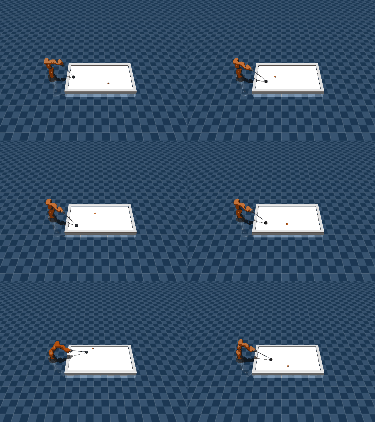
Built with
- MuJoCo
- PyTorch
- CasADi
- IPOPT
- NumPy
The problem: a game that punishes slow planners
Air hockey is a hard robotics benchmark for an unglamorous reason: the puck is faster than your control loop would like. A puck struck at ~1.5 m/s crosses the half-table in under 300 ms. A 7-DOF arm at 50 Hz gets roughly 15 control steps to observe the trajectory, plan an interception, and drive the mallet into position — with joint-velocity and workspace constraints the whole time.
This project addresses the Air Hockey Challenge 2023 (University of Freiburg), a standardised competition where a KUKA LBR iiwa14 robot arm must play three tasks in MuJoCo simulation:
| Task | Goal |
|---|---|
| Defend | Prevent the puck from entering the agent’s goal |
| Hit | Strike the puck into the opponent’s goal |
| Prepare | Push a stationary puck into a target preparation zone |
The constraints that make each task hard:
- Contact dynamics — mallet-puck impact is brief and stiff; approach angle matters.
- Workspace — the mallet must stay on the table plane ( m) inside m, m.
- Joint limits — the KUKA has per-joint position and velocity bounds that cannot be violated without hardware damage.
- Latency — a trajectory planned for where the puck was is wrong by the time it executes.
Architecture overview
Rather than choosing between model-based and learned control, the project tests two hybrids that share the same high-level policy but differ in the low-level trajectory executor.
Observation (23-dim)
        │
        ▼
  TQC Policy (2D action)      ← same in both variants
        │
        ▼
 desired (x, y) on table
        │
   ┌────┴────┐
   │         │
  IK        MPC
   │         │
   ▼         ▼
joint pos  joint vel commands → robot (50 Hz)
Shared component — TQC actor: the RL policy outputs a 2D normalised target position on the table. It learns what to aim for given the puck and arm state.
IK variant: converts the 2D target to joint angles in ~1 ms using the closed-loop IK solver built into MuJoCo.
MPC variant: solves a constrained nonlinear optimisation over a 5-step horizon in ~20 ms, explicitly encoding joint-velocity limits and workspace bounds into the trajectory.
Background: Truncated Quantile Critics (TQC)
TQC is a distributional extension of Soft Actor-Critic. Instead of maintaining a single scalar , it maintains an ensemble of critics each outputting a set of quantile estimates — a full return distribution. Over-optimism is controlled by trimming the top quantiles during target computation.
Policy representation
The actor is a Gaussian policy with a tanh squashing transformation:
Because tanh squashes to , the log-probability requires a Jacobian correction:
where is the standard normal density. The second term is numerically stabilised as:
Distributional critic
Each of critic networks outputs quantile estimates that collectively represent , the CDF of returns. The quantile targets are for .
Bellman target with top-quantile dropping: to reduce over-estimation bias, the top quantiles per network are discarded before computing targets, leaving target quantiles. Sorted and filtered:
The Bellman target for each surviving quantile is:
Quantile Huber loss
The critic is trained with asymmetric Huber regression. Let be the TD error between target quantile and predicted quantile :
where is the Huber loss with threshold :
Total critic loss, averaged over the batch and summed over predicted/target quantile pairs:
The asymmetric weight enforces that quantile underestimates at rate and overestimates at rate , which is the defining property of quantile regression.
Actor loss and automatic entropy tuning
The actor maximises the expected soft return:
where is the mean over all critic quantiles. The temperature is tuned automatically to enforce a minimum entropy target :
Target critic weights are updated via Polyak averaging at each step:
Variant 1: TQC + Inverse Kinematics
Inverse kinematics answers the question: given a desired end-effector (EE) position, what joint configuration achieves it?
The robot’s forward kinematics defines the EE position as:
The IK problem is to find satisfying . MuJoCo’s built-in CLIK (Closed-Loop Inverse Kinematics) solver iterates:
where is the damped pseudo-inverse of the Jacobian , and is a small damping constant.
Execution flow per step:
- TQC outputs .
- Rescale to physical coordinates: , .
- Set m (table surface height).
- Solve IK → joint configuration .
- Send as the position command to the robot.
Why IK is fast: the CLIK solve converges in a few iterations with no inequality constraints. Typical wall-clock time is ~1 ms per step at 50 Hz — well within budget.
Where IK falls short: IK finds a pose, not a trajectory. It does not consider joint velocity limits between the current configuration and , nor does it look ahead more than one step. In practice this can produce abrupt torques or step into configurations that are hard to escape.
Variant 2: TQC + Model Predictive Control
MPC replaces the single-step IK solve with a receding-horizon optimisation that explicitly enforces constraints over future time steps.
Why a horizon helps
At each 20 ms control step, MPC plans a short trajectory:
now      +20ms    +40ms    +60ms    +80ms    +100ms
 │         │        │        │        │         │
 s₀ ──u₀──► s₁ ──u₁──► s₂ ──u₂──► s₃ ──u₃──► s₄ ──u₄──► s₅
All five joint-velocity commands and all five EE positions are optimised simultaneously. Only is executed; the problem is re-solved next step with updated state. This means:
- Joint-velocity limits are respected across every future step, not just the current one.
- Workspace bounds are enforced as hard constraints on every .
- Anticipatory smoothing — the planner avoids configurations that would force large corrections later.
System dynamics
The EE velocity is related to joint velocities by the Jacobian:
is computed numerically at the current joint configuration via MuJoCo’s mj_jacBody. This linearisation is re-computed at every MPC call, making the approach “linearise-and-optimise” rather than globally nonlinear.
RK4 integration
Euler integration would accumulate drift. The MPC uses fourth-order Runge-Kutta for accurate rollout within the horizon:
where and s. RK4 is fourth-order accurate in , meaning integration error is per step — negligible over a 5-step horizon.
Nonlinear programme (NLP) formulation
The MPC solves, at each step:
where is the 3D target provided by TQC, and denotes one RK4 step. The workspace set is m.
KUKA LBR iiwa14 joint velocity limits (rad/s):
| Joint | ||
|---|---|---|
| 1 | −1.484 | +1.484 |
| 2 | −1.484 | +1.484 |
| 3 | −1.745 | +1.745 |
| 4 | −1.309 | +1.309 |
| 5 | −2.269 | +2.269 |
| 6 | −2.356 | +2.356 |
| 7 | −2.356 | +2.356 |
NLP variable layout. CasADi assembles the decision vector by interleaving state and control nodes:
for this gives 53 decision variables. The problem is solved by IPOPT (Interior Point OPTimizer) in typically 10–20 iterations. The first control action is extracted and applied; joint positions are integrated forward:
Why MPC outperforms IK
The table below captures the key trade-offs:
| Property | IK | MPC |
|---|---|---|
| Planning horizon | 1 step (greedy) | 5 steps (0.1 s) |
| Joint velocity constraints | Implicit — may saturate | Explicit — never violated |
| Workspace constraints | None | Hard inequality constraints |
| Trajectory smoothness | Potentially jerky | Smooth by construction |
| Per-step compute | ~1 ms | ~20 ms |
| Solver success rate | ~100 % | ~99 % (IPOPT convergence) |
The key insight is predictive constraint satisfaction. IK generates the nearest joint configuration that reaches the target — if the required motion exceeds a joint velocity limit, the robot simply saturates and falls short. MPC, by contrast, solves for the entire trajectory simultaneously. If the target requires fast motion in a direction where a joint is near its limit, the optimiser redistributes the workload across the other six joints over the full horizon.
Receding-horizon planning prevents local traps. A greedy controller (IK) can move the arm into a configuration that is excellent for the current step but constrains every subsequent step — for example, parking a joint near its limit to intercept one puck, then being unable to recover for the next shot. MPC sees 100 ms ahead and implicitly penalises ending the horizon in a poor posture.
Smoothness emerges from the cost, not from filtering. IK outputs are sometimes post-processed with filters to reduce jitter. MPC produces smooth trajectories without post-processing because continuity is encoded in the dynamics constraints — must be reachable from under the RK4 model, which already limits how fast the EE can jump.
The cost for this is the ~20× higher per-step compute (~20 ms vs ~1 ms). On the defend task this is affordable at 50 Hz, but would become a bottleneck in faster tasks or on hardware with tighter real-time guarantees.
Reward design
The reward functions are designed to be sparse at the terminal level (large bonus/penalty at episode end) and dense during execution (continuous shaping terms that guide early learning).
Defend reward
Phase 1 — Approach (before first mallet-puck contact):
where is the point on the defensive line with the same -coordinate as the puck.
Phase 2 — Post-contact (after the mallet touches the puck, if puck moves toward agent):
This rewards slowing the puck’s horizontal velocity.
Terminal rewards:
Constraint violation penalty (soft, applied every step):
summed over all joint position, velocity, and workspace violations. This soft penalty encourages feasibility during training without hard resets.
Hit reward
The hit task requires striking the puck toward the opponent’s goal, so the reward encodes both approach angle and post-contact velocity:
where — the agent may aim directly or use a bank shot.
Post-contact:
The posture penalty discourages drifting into awkward configurations after the strike. Terminal: if the puck scores.
Prepare reward
The agent must push the puck into the preparation zone . A symmetric approach-angle reward guides the mallet to contact the puck from a direction pointing into . Terminal: if puck is in at episode end, otherwise.
Training setup
Both agents share the same hyperparameters and training pipeline.
| Hyperparameter | Value |
|---|---|
| Algorithm | TQC |
| Total timesteps | 50 M |
| Discount | 0.99 |
| Polyak | 0.005 |
| Batch size | 256 |
| Actor/critic LR | |
| Temperature LR | |
| Critic networks | 5 |
| Quantiles per net | 25 |
| Top quantiles dropped | 2 |
| Max episode steps | 500 (10 s) |
| Evaluation frequency | every 3 000 steps |
Replay buffer: standard FIFO with capacity transitions. Each transition stores where : puck position (3), puck velocity (3), joint positions (7), joint velocities (7), opponent EE position (3).
Gradient updates: one update per environment step, sampling a fresh batch each time. Critic and actor losses are back-propagated separately; target critics are updated with Polyak averaging after each step.
Environment
Simulation: MuJoCo (stiff contact dynamics, required for accurate mallet-puck collisions).
Control frequency: 50 Hz ( s).
Robot: KUKA LBR iiwa14, 7 degrees of freedom.
Table geometry:
| Parameter | Value |
|---|---|
| Length | 1.948 m |
| Width | 1.038 m |
| Goal width | 0.25 m |
| Surface height | 0.1645 m |
Observation space (23 dimensions):
| Component | Dim | Description |
|---|---|---|
| Puck position | 3 | in world frame |
| Puck velocity | 3 | |
| Joint positions | 7 | (rad) |
| Joint velocities | 7 | (rad/s) |
| Opponent EE | 3 | of opponent mallet |
Action space: 2D Cartesian target normalised to .